
Making Progress in Seattle’s Urban Forest
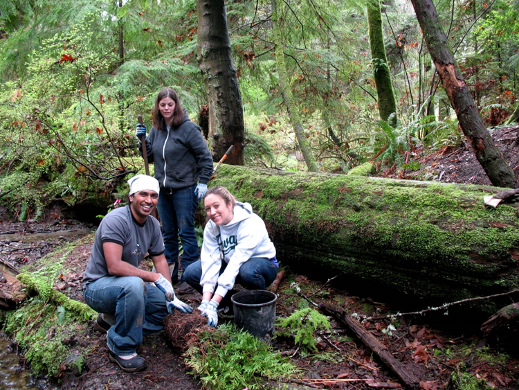
I recently returned to one of the sites at Schmitz Preserve Park where I led habitat restoration over a decade ago, and I’ll be honest, the site is a total mess. It seemed so simple in the beginning. Remove the weeds and plant native trees. What happened?
At the time, I was a college student volunteering as a GSP Forest Steward for my senior capstone project. Bright eyed and bushy tailed, I had an impossibly optimistic vision for the site. It would be an outdoor learning space for the nearby schools. Edible native plants would grace the edges of the sidewalk, and racoons would nap in the nooks of the trees that I had planted. In the soil, a rejuvenated network of mycelium would nourish the plants with water drawn from deep underground during the parched summer drought season.
I still think that vision has potential, but after I graduated from college and moved on to other adventures, the continuity of care at the site was broken. Not only did the Himalayan blackberry bounce back, but there were new weed species that started popping up – bindweed and creeping buttercup in the sheet-mulched areas, nipplewort and shotweed in the disturbed soil, and poison hemlock along the fence line by the elementary school. I felt like I had opened Pandora’s proverbial box of weeds, and I didn’t understand why.
Did other restoration projects also see an increase in weed diversity over time? Was there an optimum number of maintenance hours needed to keep the weeds down? And was there something about the work itself that, perhaps counterintuitively, may have degraded the site or encouraged the weeds to grow?
Green Seattle Partnership’s Forest Monitoring Program aims to unravel some of these questions about why different outcomes occur at our ecological restoration projects. As part my work at Haven Ecology and Research LLC, I recently had the opportunity to support Seattle Parks and Recreation and the Green Seattle Partnership with additional data collection and analysis. We explored how the structure and diversity of our urban forest has changed over the last decade by comparing data before and after two particular management actions: weed removal and plant installation.
A Citywide Network of Monitoring Plots
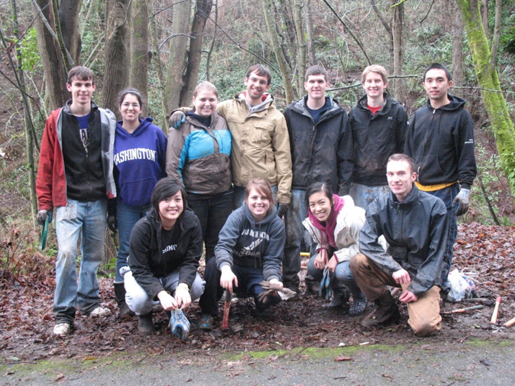
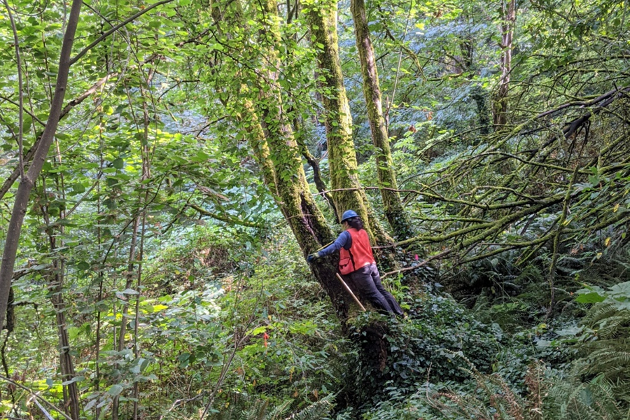
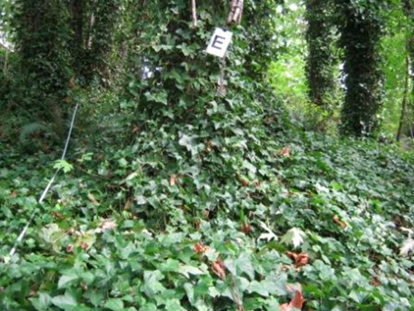
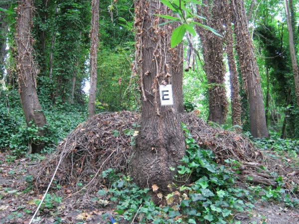
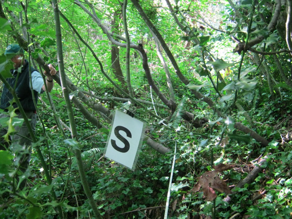
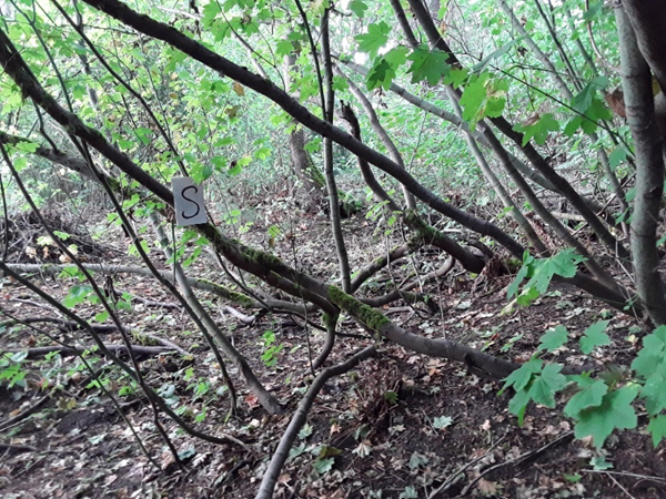
At that very site that I cared for in Schmitz Preserve Park, hidden between some ferns, there is a metal post hammered into the ground, marking the center of a permanent monitoring plot. This plot is one of hundreds throughout Seattle where teams of community scientists and professional crews have returned, over and over, to gather information about forest structure, plant diversity, soil quality and many other site characteristics related to forest health.
The GSP Forest Monitoring Program plays a key role in fulfilling the Green Seattle Partnership’s long-term goals outlined in the strategic plan. By collecting information about how the urban forest changes over time, we can track progress, prioritize resources, and develop insight into what works.
Forest Monitoring Protocol Summary
- 1/10-acre permanent plots
- Measure the height and diameter of all trees over 4.5 ft tall.
- Measure the height of all trees under 4.5 ft tall.
- Visually estimate the percent cover of each understory species.
- Collect information on site characteristics (aspect, slope, coarse woody debris, canopy cover, soil compaction, etc.)
- Document the location of the plot center with rebar center post, photos, walking directions, witness objects and latitude/longitude coordinates.
Weed Cover is Decreasing
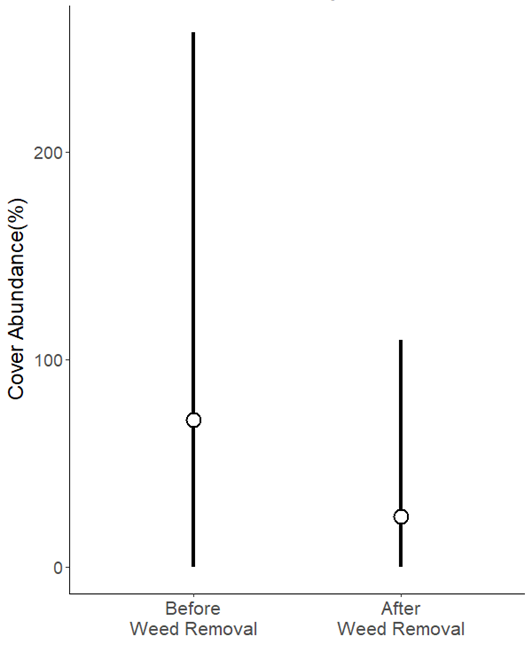
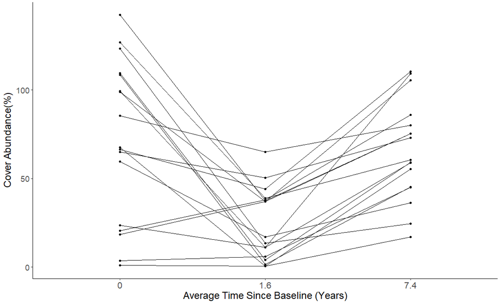
Some of the most dramatic and visible changes in the urban forest follow the removal of weed species that often dominate a site. The monitoring data show that the average cover-abundance of weed species decreased from 71% to 25% (p < 0.001) following initial removal. Those numbers are reason enough for a celebratory nod, but it gets even better when we realize that those averages are skewed a bit high due to outliers that pull the average value up. Some restoration sites begin with a cumulative weed cover as high as 250%. This can happen when there are multiple weed-species overlapping each other at a site, such as a layer of ivy under a layer of blackberry under a layer of clematis in the canopy.
And yet, in some places, weed cover remains surprisingly high following initial restoration work – up to 100% at some plots. What’s going on in cases like this?
| A quick note about statistics: For hypothesis testing, we used a statistical test known as the paired-sample t-test to help us determine whether the changes over time were noteworthy, with a p-value below 0.01 indicating statistically significant differences. This is a very simplified analysis of what is actually a pretty complex and nonlinear process of ecological repair. Nonetheless, we use “before and after” comparisons like this to see what we can learn from sites where ecological restoration is underway. |
Firstly, we must apply some healthy skepticism to the data itself. It is always possible that a person may have over-estimated the weed cover at some plots. However, these outliers may also represent areas where restoration work was initiated but, for one reason or another, the continuity of stewardship was broken, allowing the weeds to bounce back. Some monitoring plots have enough time points that we can catch a glimpse of what happened at these outliers. At many of these plots, we see that dramatic decreases in weed cover did indeed occur, but that weed cover has increased since then. A handful of other plots appear to have had little to no change in weed cover over time.
| Cover-abundance A metric describing the abundance or extent of a species, represented as the percentage of a given area that it occupies (also called percent cover). See the end of the post for additional terms and definitions. |
Although these outliers represent just a fraction of the outcomes observed across all monitoring plots, they showcase important questions that can help us improve our adaptive management practices. How much time elapsed between the initial weed removal work and the final monitoring time point? How many person-hours of work were invested in follow-up weeding per acre? Or per year? Are some weed species more resilient than others? Each of these questions is an opportunity to explore these nuanced site histories beyond the “before and after” comparison discussed here.
Plant Diversity is Increasing
Weed removal is great and all, but what about the impacts of restoration on the biodiversity of the plant community? One way of measuring biodiversity is by calculating the species richness, which is simply the total number of species at a site. The monitoring data show that native plant species increased from an average of 9.7 to 13.5 species per plot (p < 0.001). There are a wide range of site histories hidden in those numbers though. Prior to plant installation, the species richness of native plants ranged from 2 to 31 species per plot, which is yet another reminder of just how unique each project can be. Some sites start out in a successional state approximating the diversity and structure of an old growth forest. At other sites, we may be starting from scratch with the removal of a blackberry thicket on the side of the road.
Surprisingly, the average number of non-native species has also gone up, rising from 5.0 to 6.2 species per plot (p < 0.001) following initial restoration work. It remains unclear what is driving this pattern.
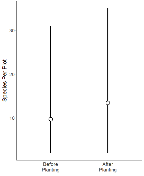
Change in the species richness of native understory plants before and after plant installation. Points represent averages and vertical lines represent minimum and maximum values. Native understory plants are increasing in species richness.
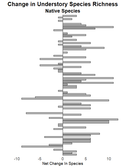
Net change in the species richness of native plants – each bar represents the most recent data from an individual plot. Native plants have increased by an average of 3.4 species per plot following initial plant installation activities. However, a minority of plots show a decline in native species diversity.

Net change in the species richness of non-native plants – each bar represents the most recent data from an individual plot. Some plots show a decrease in species, but on average, weed diversity has increased by 1.1 species per plot following initial weed removal activities.
Native Plants Take Time to Establish
Changes in the cover-abundance of native understory plants are difficult to summarize with a single statistic. Following initial plant installation, the average percent cover changed from 73% to 74%. Why don’t we see big increases in the average cover of native plants when there are concurrent declines in the cover-abundance of weed species? The simplest explanation is that it simply takes time. As many a gardener will tell you, “The first year, they sleep. The second year, they creep. The third year, they leap.” And so, it grows.
It’s also possible that at some monitoring plots, native plants were already high in abundance, with the restoration work likely involving only minor weed removal to prevent further impacts to the existing native plant community. In other cases, there are indeed dramatic increases in native plant cover following management actions. There are a wide range of site histories that tell many different stories – impossible to summarize in a statistic like an average.
The cover-abundance of native understory plants may take time to develop, but the density of regenerating trees has increased rapidly as a result of plant installation. The average density of native seedlings and saplings has increased from 138 to 234 stems per acre (p < 0.001) at sites where plant installation occurred. And it is these young regenerating trees that are so essential for the long-term sustainability of our urban forest.
Onwards and Upwards
Thinking back to the restoration site that I volunteered at so many moons ago, I know that one day someone else will take care of that site with the same impossible optimism that inspires ecological restoration all over the world. They might be a community volunteer who dedicates years of their life to the site, or they could be a professional crew member passing through for a single day. The Green Seattle Partnership is a community-driven program, and we know that continued commitment to these spaces translates to healthier forests in the long run. Meanwhile I will be out in the woods this summer collecting data for the GSP Forest Monitoring Program to help us better understand how the forest is changing over time.
About the Author
Dylan Mendenhall is the owner and principal ecologist of Haven Ecology and Research LLC, a small environmental consulting firm with a mission to help our community make strategic land use decisions. Over the years, he has worn many hats at the Green Seattle Partnership, including as a Forest Steward at Schmitz Preserve Park. While working at EarthCorps, he coordinated the GSP Forest Monitoring Program and led habitat restoration projects throughout the Puget Sound region. He has an MSc in Forestry from the University of British Columbia and a Certificate in Data Science from the University of Washington.
Additional Reading
GSP Long-Term Monitoring Tells a Story of Improving Forest Health, May 2020
The GSP Approach to Using Ecological Assessments, May 2020
Terms and Definitions
Average
A metric describing the central tendency of a set of values, calculated by adding up the values and dividing by the total number of values. Also called the mean.
Cover-abundance
A metric describing the abundance or extent of a species, represented as the percentage of a given area that it occupies (also called percent cover)
Diversity
Diversity (also called biodiversity) is the variety of living organisms in an ecosystem, both in terms of the species richness (i.e. the total number of species) and their relative abundances to each other. Diversity can be measured using a variety of metrics, including the Shannon diversity index.
Median
A metric describing the central tendency of a set of values, calculated by finding the middle value, with an equal number of values higher and lower than it.
Outlier
A term used in statistics for describing values that are unusually high or low.
Paired sample t-test
A type of statistical analysis used to provide guidance on whether a management activity or experimental treatment actually worked (also called statistical significance). A paired sample t-test compares the same locations or samples before and after the management activity occurred. The resulting p-value indicates the expected probability that the outcome happened by chance.
Regeneration
Tree regeneration is the process of a forest becoming reestablished through the growth and survival of young seedlings and saplings.
Species richness
A diversity metric representing the total number of unique species in an ecosystem. Species richness is one of many ways to quantify biodiversity.
Structure
Structure is the physical size, distribution and abundance of trees, shrubs, snags, logs and other physical parts of an ecosystem. Structure can be measured using metrics such as stems per acre or cover-abundance (%).
Wild plant seeds. Both native and weeds, stay viable in the soil for years, even decades, so I’m not surprised that you see increased species diversity often weed removal. In general, species diversity is good so I don’t see these outcomes as a failure of the program.